Time Series Project: Eye Tracking Signals and Filtering

• Project name: nsd_eye_tracking_time_series
• Research question: During repeated NSD image presentations, is gaze movement lower while the target image is on screen than during nearby periods when that target is not on screen?
• Optional extension: Does the filtered pupil-size signal change in the seconds after image onset?
• Programming language: R suggested. Python is not needed for the main workflow.
• Expert contact: TBD, Roy Hessels?

Canonical course conventions live in project_guidelines.md. That file is the source of truth for the four required workflow files (week1_explore.qmd, week2_operationalize_clean.qmd, week3_model.qmd, week4_storytelling.qmd), the data/model_data.rds -> data/model_results.rds pipeline, the raw-data policy, quality-check requirements, decision logs, and contribution tracking. Read it before starting and treat anything below as project-specific guidance on top of those conventions.

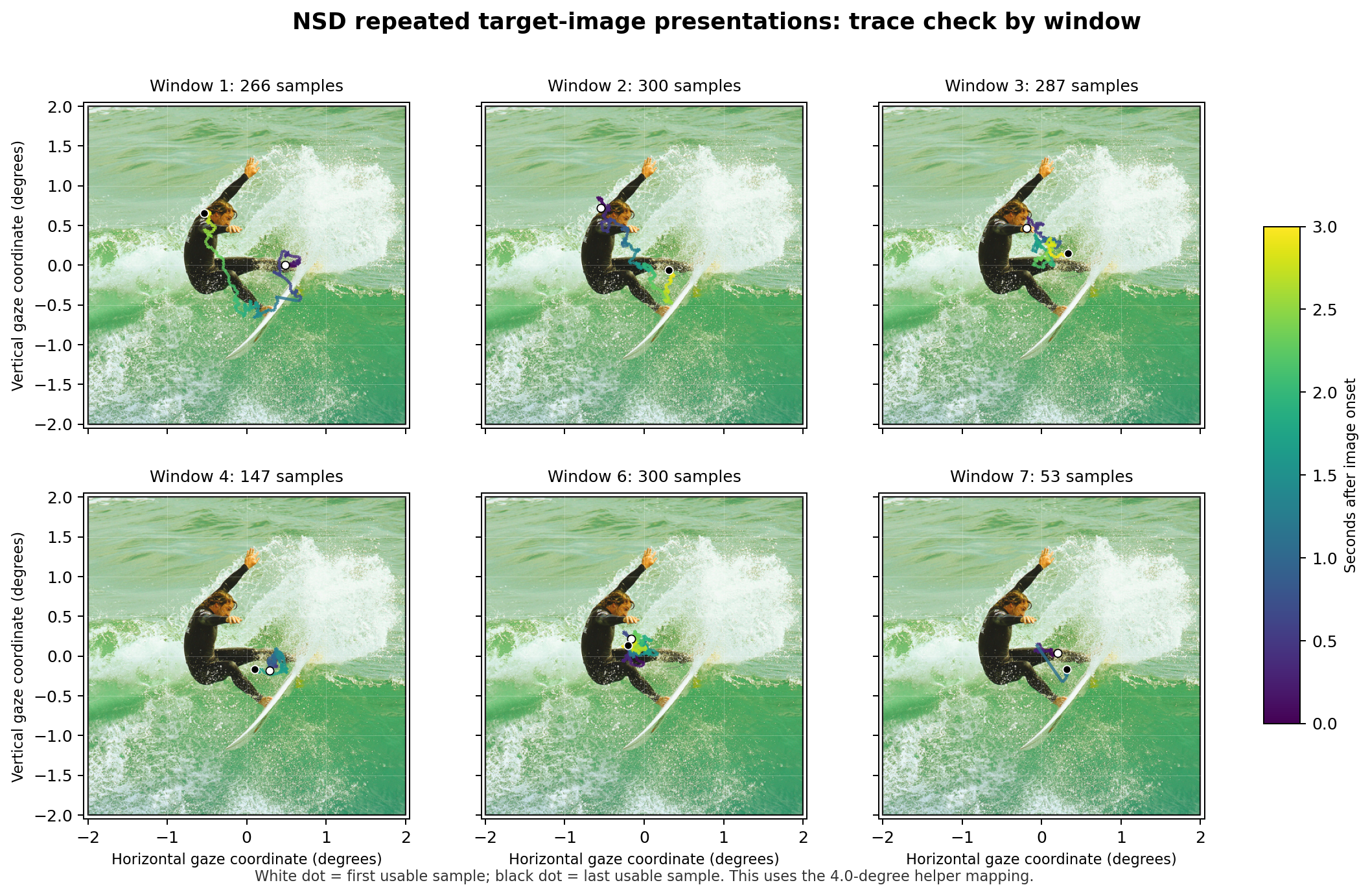
Example from an NSD eye-tracking run: gaze traces from six usable 3-second repeated presentations of the same target image. Each panel maps gaze onto the actual image as a 4.0 x 4.0 degree square, matching the helper relationship x_plot = (x + 2) / 4 and y_plot = (2 - y) / 4. Color shows seconds after image onset; white and black dots mark the first and last usable samples.

Tutorial framing

Eye-tracking is a good time-series project because the raw object is a dense signal: time, horizontal gaze, vertical gaze, pupil area, blinks, saccades, and task messages. The small scientific question is about movement during image viewing. The programming lesson is how to turn raw signal files into a regular, filtered, event-aligned time series.

Students should learn four things:

1. How eye-tracking data are represented as samples, event intervals, task messages, device-specific files, and inspection plots.
2. Why file formats matter: raw EyeLink EDF files, NSD’s MATLAB .mat preprocessing, and a student-created RDS cache expose different parts of the provenance chain.
3. How filters work on a noisy signal. Students should compare a raw trace with at least two simple filters, then choose one filter for the analysis.
4. How to fit a tiny time-series model that accounts for autocorrelation instead of pretending each sample is independent.

The core research question is intentionally modest:

Is the filtered gaze-velocity signal lower during target-image viewing windows than during nearby periods when that target is not on screen?

The project should not become a full psychology project about why someone looked at a particular surfer, object, or region. It should also not make preprocessing the research question. Filtering is part of the method. A filter-width change can be a sensitivity check, but the main question is about gaze movement during an experimental event.

The fixation/saccade literature is still useful, but mainly as a warning about language. If students label low-velocity periods, they should call them computational candidates and report the rule. They should not claim that their code has discovered true fixations.

Peer-teaching checklist

Dimension	This project teaches
Data structure	Regularly sampled gaze and pupil time series, missing samples, event windows, blink/saccade intervals, and run-level metadata.
Storage system	Scientific repository on AWS plus a small local RDS cache created from the NSD MATLAB file.
File formats	EyeLink .edf, MATLAB .mat, JPG inspection plots, PNG stimulus images, and RDS/CSV outputs created by students.
Encoding	Binary eye-tracker files, MATLAB arrays, numeric time-series tables, and image-based quality-control plots.
Model	A small AR(1)/ARIMA-style model with an event indicator: filtered gaze velocity as the outcome and image_on as an external regressor.
Key aspects to explain	Sampling rate, missing samples, blinks, filtering, velocity, event alignment, autocorrelation, AR(1) errors, aggregation to 100 ms bins, one continuous modeling segment, and sensitivity to one filtering choice.

Resources

Data source

Use the Natural Scenes Dataset (NSD) eye-tracking data so this project shares provenance with the neuroimaging project but teaches a different data structure. NSD access requires accepting the NSD data terms.

Start with one subject, one run, and one repeated target image. A good teaching subset is:

• Preprocessed subject-level MATLAB file: s3://natural-scenes-dataset/nsddata_timeseries/ppdata/subj01/eyedata_preprocessed.mat
• Raw EyeLink folder to list and discuss, not fully parse: s3://natural-scenes-dataset/nsddata_timeseries/ppdata/subj01/eyedata/
• Eye-tracking inspection plots: s3://natural-scenes-dataset/nsddata/inspections/eyetrackinginspections/pupil_subj01_nsdimagery_run01.jpg and s3://natural-scenes-dataset/nsddata/inspections/eyetrackinginspections/XY_subj01_nsdimagery_run01.jpg
• NSD imagery design files: s3://natural-scenes-dataset/nsddata/experiments/nsdimagery/designmatrixGLMsingle.mat and the relevant pair-list file, such as B_pair_list.mat
• One or a few small target images from: s3://natural-scenes-dataset/nsddata/experiments/nsdimagery/rawtargetimages/

Here “repeated target image” means that the same stimulus appears multiple times within the run. In the example figure, shared0385_nsd28752.png is scheduled at eight separate onsets in run 2. Each onset starts a 3-second image-presentation period, followed by a 1-second rest/fixation period. These are repeated presentations of the same image, not eight different screen regions.

Do not download the full 37 GB nsd_stimuli.hdf5, all subjects, all EDF files, or any fMRI beta files for this project.

The raw .edf files are the device-native EyeLink recordings. They are important for provenance and for the Week 1 open-format discussion. They are not the recommended main input because direct EDF parsing in R adds too much tool friction. The .mat file is the practical starting point because it preserves the time-series structure students need while keeping the course workflow small.

Knowledge sources

• Roy Hessels and Ignace Hooge PEP assignments 6 and 7: gaze traces, velocity, filtering, and careful inspection.
• Hessels et al. (2018), “Is the eye-movement field confused about fixations and saccades?”, for the warning that fixation/saccade definitions must be explicit.
• Hooge et al. (2022), “Fixation classification: how to merge and select fixation candidates”, for why selection rules should be reported if candidates are used.
• R packages: R.matlab, dplyr, tidyr, ggplot2, readr.
• Useful base R functions: diff(), stats::filter(), stats::runmed(), stats::acf(), stats::arima(), is.finite(), and aggregate().
• Optional package if students want a more familiar ARIMA interface: forecast.

Filter choices

Students should learn what filters do before applying one:

• A moving average smooths high-frequency jitter but blurs fast movements and creates edge artifacts.
• A median filter is robust to isolated spikes but can flatten sharp changes.
• A low-pass filter keeps slow movement and removes fast jitter, but students must explain the cutoff frequency if they use one.

For the class version, require one simple filter for the final analysis. A centered moving average over 5 to 11 samples is enough. The sensitivity check can be a second window width, not a large preprocessing contest.

Week-by-week

Week 1

Start from the AWS repository and the downloaded .mat file. The goal is to understand what the raw scientific object is before filtering anything.

Week 1 exact data checklist:

• Read and accept the NSD data terms.
• Download eyedata_preprocessed.mat for subj01.
• Download the two inspection JPGs for one run.
• List the raw EDF folder, but do not download every EDF file.
• Download only the small nsdimagery design/pair-list files needed to identify one repeated target-image window.
• Download one small target PNG if the group wants to make an overlay.
• Save a small cached extract such as data/model_data.rds only after students have documented which raw fields it came from.

Week 1 questions:

• What is one row in the sample table?
• What is the sampling rate after preprocessing?
• Which columns represent time, x gaze, y gaze, and pupil area?
• Which file tells us when the target image is on screen?
• What is a target-image presentation, and how is it different from a screen region or image file?
• What does the device-native EDF file preserve, what does the NSD .mat preprocessing make easier, and what are the consequences of relying on proprietary binary formats rather than open, documented, analysis-ready formats?
• Which data are samples, which are events, and which are inspection plots?

Prepare for roundtable in week 2:

• Explain why eye tracking is a time-series data structure rather than an independent-row table.
• Explain the provenance chain EDF -> .mat -> RDS. Which decisions are visible at each step, and which are harder to audit?
• Explain why blinks and tracking loss are not ordinary missing values.
• Explain why a project can analyze gaze velocity without claiming to classify true fixations or saccades.

Week 2

Operationalize the research question by building one small, regular time-series table.

• Choose one subject and one run.
• Use the nsdimagery design file to create an image_on indicator for the selected target-image windows.
• For plotting, keep small event windows around presentations, such as 3 seconds before image onset through 3 seconds after image offset.
• For the AR(1) model, keep one continuous segment spanning the first selected target onset through the last selected target offset, plus a small margin. Do not paste separate event windows together and then treat them as adjacent time points.
• Convert time to seconds from run start.
• Mark valid samples where x, y, and pupil area are finite.
• Compute gaze displacement and velocity from x/y using diff().
• Aggregate or resample to 100 ms bins to keep the model small.
• Plot raw velocity and at least two filtered versions.
• Choose one filter for the final model, such as an 11-sample moving average.
• Create log_velocity_filtered = log1p(velocity_filtered) so the highly skewed velocity signal is easier to model.
• Save data/model_data.rds with only the columns needed for Week 3: time_sec, event_id, time_from_onset, image_on, valid_fraction, velocity_raw, velocity_filtered, log_velocity_filtered, and optional pupil_filtered.

Prepare for roundtable in week 3:

• Explain what each filter did to the trace and why the chosen one is reasonable.
• Explain why filtering can remove jitter but can also blur fast movements.
• Explain how the image_on variable was made from the design file.
• Explain why nearby periods from the same continuous run are a better comparison than unrelated parts of the recording.

Week 3

Fit a small time-series model. Do not fit ordinary sample-level OLS as the main model, because adjacent samples are autocorrelated.

Recommended model:

fit_data <- model_data[
  is.finite(model_data$log_velocity_filtered) &
    is.finite(model_data$image_on),
]

fit <- arima(
  fit_data$log_velocity_filtered,
  order = c(1, 0, 0),
  xreg = fit_data$image_on
)

Here order = c(1, 0, 0) is an AR(1) model: the current value is allowed to depend on the previous value. The image_on coefficient answers the simple research question. A negative coefficient means gaze movement is lower while the target image is on screen, after accounting for short-range autocorrelation. Use a continuous, equally spaced time series for this model. Event-aligned windows are useful for visualization, but they should not be concatenated for the AR(1) fit.

Students should also show:

• the autocorrelation plot of log_velocity_filtered;
• a naive mean difference for intuition;
• the AR(1) estimate for image_on;
• one sensitivity check using a different filter width.

Avoid a black-box auto.arima() search unless the group can explain why it chose the final model. A fixed AR(1) is enough for this course.

Prepare for roundtable in week 4:

• Explain what autocorrelation means in this signal.
• Explain why an AR(1) model is already more time-series-aware than ordinary OLS.
• Explain which parameter answers the research question.
• Explain what changed, if anything, when the filter width changed.

Week 4

Visualize and tell a story about the time-series pipeline.

• Show the raw gaze trace or velocity trace.
• Show the chosen filtered trace.
• Show the target-image windows as shaded regions on the time axis.
• Show the event-aligned average of filtered velocity around image onset.
• Show the AR(1) model result in plain language.
• Optionally show the gaze overlay on the target image as a sanity check.

The final story should make a course-level argument:

A time-series result is not only a model output. It depends on the raw file format, sampling rate, missing-data handling, filtering, event alignment, autocorrelation, and the exact comparison window.