Scientific Programming Project: Neuroimaging Data Standards
- Project name:
scientific_programming_neuroimaging - Research question: In NSD subject 1, session 1, is the mean beta response different in V1 and hV4?
- Optional extension: If the core pipeline works, repeat the same ROI comparison for a few additional sessions or revisit the V1 session-drift question.
- Programming language:
Rsuggested for the class version (RNifti,dplyr,tidyr,ggplot2). Python remains optional for students who already knownibabelornilearn. - Expert contact: TBD, Ben Harvey?
Canonical course conventions live in project_guidelines.md. That file is the source of truth for the four required workflow files (
week1_explore.qmd,week2_operationalize_clean.qmd,week3_model.qmd,week4_storytelling.qmd), thedata/model_data.rds->data/model_results.rdspipeline, the raw-data policy, quality-check requirements, decision logs, and contribution tracking. Read it before starting and treat anything below as project-specific guidance on top of those conventions.
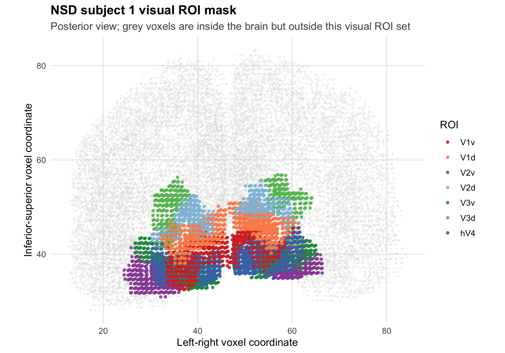
Posterior view of an NSD visual ROI mask: grey points are valid brain voxels outside this visual ROI set; colored points show V1, V2, V3, and hV4 subdivisions. The practical task is to connect voxel coordinates, ROI labels, trials, and beta values into one small analysis table.
Tutorial framing
This project is about scientific data standards and binary scientific arrays. The raw object is not one tidy table. It is a small set of files that only make sense together: BIDS metadata, JSON sidecars, event TSV files, NIfTI beta maps, ROI masks, and a dataset manual.
The project should stay deliberately small. Students should not try to do a full fMRI study, fit a complex neural encoding model, download all NSD sessions, or solve image-category labeling. The class version uses one subject, one session, one single-trial beta file, and one visual ROI mask.
Students should learn three things:
- How a scientific repository uses standards and metadata to make a large dataset understandable.
- How a NIfTI beta file and a NIfTI ROI mask encode different but aligned arrays.
- How to reduce voxelwise trial data to a small trial-by-ROI table that answers one simple question.
The core research question is:
Are mean trial-level beta responses different in V1 and hV4 for one NSD subject-session?
This is not meant to be a new neuroscience contribution. It is a defensible mini-question that forces students to work with real neuroimaging files without drowning in the full NSD dataset.
Peer-teaching checklist
| Dimension | This project teaches |
|---|---|
| Data structure | Participant/session folders, event metadata, 4D beta images, 3D ROI masks, voxel coordinates, trial index, and ROI labels. |
| Storage system | Scientific repository on AWS organized through BIDS-style and NSD-specific conventions. |
| File formats | NIfTI .nii.gz, TSV, JSON, CSV, MATLAB design files if needed, and RDS/CSV outputs created by students. |
| Encoding | Text metadata, JSON sidecars, tabular event files, binary scientific image arrays, and integer-coded ROI masks. |
| Model | A paired trial-level ROI comparison, such as a one-sample test or bootstrap interval for hV4 - V1 trial differences. |
| Key aspects to explain | Data standards, provenance, voxel-to-ROI mapping, NIfTI dimensions, trial indexing, ROI aggregation, file sizes, and what is lost when voxel maps become ROI means. |
Resources
Data source
The practical uses the Natural Scenes Dataset (NSD). European fMRI datasets are difficult to share publicly because detailed brain images are often treated as individually identifiable under the GDPR. NSD is an American dataset that can be shared through AWS Open Data after signing the NSD data access agreement.
- Dataset and documentation: https://naturalscenesdataset.org/
- Main reference paper: Allen et al. (2022), Nature Neuroscience. https://doi.org/10.1038/s41593-021-00962-x
- Optional extension reference for session drift: https://doi.org/10.1038/s41467-023-40144-w
Minimum NSD files for the class version:
- BIDS metadata:
nsddata_rawdata/dataset_description.json,nsddata_rawdata/participants.tsv, andnsddata_rawdata/task-nsdcore_bold.json. - One example event file:
nsddata_rawdata/sub-01/ses-nsd01/func/sub-01_ses-nsd01_task-nsdcore_run-01_events.tsv. - Subject 1 visual ROI mask:
nsddata/ppdata/subj01/func1pt8mm/roi/prf-visualrois.nii.gz. - One single-trial beta file:
nsddata_betas/ppdata/subj01/func1pt8mm/betas_fithrf_GLMdenoise_RR/betas_session01.nii.gz. - Stimulus metadata only for inspection, not for the core model:
nsddata/experiments/nsd/nsd_stim_info_merged.csv. - Optional image examples:
a few files from
nsddata_stimuli/stimuli/nsd/shared1000/.
Students should not download all raw BOLD volumes, all subjects, all sessions of
single-trial betas, or the full 37 GB nsd_stimuli.hdf5 file. If laptop storage
or memory is a problem, the instructor can provide a pre-cropped subset or let
students use meanbeta_session01.nii.gz for Week 1 exploration only. The main
Week 2 table should still be built from a documented NIfTI beta file plus the ROI
mask.
ROI codes
These ROI labels are retinotopic visual cortex regions: mapped areas near the back of the brain, mostly in occipital cortex, that respond to visual information. They are not arbitrary labels. They tell students which voxels belong to early visual-processing areas.
| ROI label | Brain area | Very short interpretation |
|---|---|---|
V1v / V1d |
Primary visual cortex, ventral/dorsal parts | First major cortical stage of visual processing; sensitive to edges, orientation, contrast, and spatial layout. |
V2v / V2d |
Secondary visual cortex, ventral/dorsal parts | Early visual processing beyond V1; involved in contours, texture, and figure-ground organization. |
V3v / V3d |
Third visual area, ventral/dorsal parts | Intermediate visual features, including aspects of form, motion, and depth. |
hV4 |
Human V4, ventral occipital visual cortex | Often associated with color, shape, and object-related visual processing. |
Here, v means ventral and d means dorsal. For example, V1v is the
ventral portion of V1 and V1d is the dorsal portion of V1. The class project
does not require students to make strong neuroscience claims from these labels;
the main goal is to learn how a voxel-level ROI mask links brain coordinates to
an analysis table.
For the core question, combine:
- V1 = ROI codes
1and2(V1v,V1d) - hV4 = ROI code
7
Students do not need to analyze every ROI. They should understand that the ROI mask is an integer-coded spatial map whose dimensions must align with the beta file’s spatial dimensions.
Knowledge sources
- BIDS documentation for neuroimaging data organization and metadata.
- Basic introductions to NIfTI, JSON sidecars, events files, and participant metadata.
- NSD documentation, the main paper, and the dataset manual.
- R packages:
RNifti,dplyr,tidyr,ggplot2,readr. - Optional Python equivalents:
nibabel,numpy,pandas,nilearn.
Week-by-week
Week 1
Start from the raw scientific repository, identify the files that belong together, and make a written manifest before downloading large files.
Week 1 exact data checklist:
- Read and accept the NSD data terms.
- Download only the BIDS metadata files listed above.
- Download one event TSV for
sub-01,ses-nsd01,run-01. - Download the subject-1 visual ROI mask.
- Download one selected beta file, preferably
betas_session01.nii.gz. - Optionally download a few
shared1000images so the group can see what kind of stimuli were used. - Save a local manifest with file paths, file sizes, and the reason each file is needed.
- In R, load only the headers first and write down the dimensions of the ROI mask and beta file.
Skip in Week 1:
- all raw BOLD fMRI volumes;
- all subjects;
- all beta sessions;
- the full
nsd_stimuli.hdf5; - animate/inanimate labeling;
- session-drift modeling.
Week 1 questions:
- What is BIDS, what is NIfTI, and what is a JSON sidecar?
- What is a voxel?
- What does each dimension of the beta file represent?
- What is an ROI mask, and why are most voxels outside this visual ROI set?
- Which files are raw measurements, which are metadata, and which are derived analysis files?
- Why is the data-use agreement part of the scientific data structure?
Prepare for roundtable in week 2:
- Explain why scientific data standards exist.
- Explain the difference between an event TSV, a beta NIfTI file, and an ROI mask.
- Explain why a binary array is not self-explanatory without metadata.
- Explain what can go wrong if the beta file and ROI mask dimensions do not match.
Week 2
Build the smallest useful analysis table from the raw files.
- Load the ROI mask with
RNifti::readNifti(). - Load the beta file with
RNifti::readNifti(). - Confirm that the first three beta dimensions match the ROI mask dimensions.
- Create a voxel table only for V1 and hV4 voxels.
- For each trial, compute the mean beta in V1 and the mean beta in hV4.
- Save
data/model_data.rdswith columns such as:subject,session,trial,roi,n_voxels, andmean_beta.
The Week 2 output should be small. Students should not save a copy of the full NIfTI array as an RDS file.
Prepare for roundtable in week 3:
- Explain how voxelwise maps became a trial-by-ROI table.
- Explain what was gained and lost by averaging over voxels.
- Explain why V1 was built from
V1vandV1d. - Explain one quality check: dimensions match, non-empty ROIs, plausible number of trials, or no all-missing beta summaries.
Week 3
Fit a very small model on the Week 2 table.
Recommended analysis:
wide <- tidyr::pivot_wider(
  model_data,
  names_from = roi,
  values_from = mean_beta
)

wide$hV4_minus_V1 <- wide$hV4 - wide$V1
t.test(wide$hV4_minus_V1)
Equivalent model:
lm(hV4_minus_V1 ~ 1, data = wide)
The intercept is the average trial-level difference between hV4 and V1. This is simple enough to explain and still depends on the real scientific-programming work: students had to read NIfTI files, decode the ROI mask, align dimensions, and aggregate a 4D array into a table.
Sensitivity check:
- Repeat the comparison with
V1vandV1dseparately, or - repeat after removing trials with extreme beta values, or
- repeat with
meanbeta_session01.nii.gzas a descriptive check only.
Prepare for roundtable in week 4:
- Explain which parameter answers the research question.
- Explain why the model is small but the data processing was not trivial.
- Explain why trial-level values are not the same as raw BOLD time series.
- Explain why session drift and image-category questions are extensions, not the core project.
Week 4
Visualize and tell a story about the raw-data-to-table pipeline.
- Show the ROI mask image or 3D ROI plot.
- Show the distribution of trial-level mean beta values for V1 and hV4.
- Show paired trial differences or a confidence interval for
hV4 - V1. - Show the local file manifest and the final
model_data.rdsstructure. - Make the limitations explicit: one subject, one session, two ROIs, ROI means rather than voxelwise modeling, and no claim about all visual cortex or all people.
The final story should make a course-level argument:
Scientific programming is not just fitting a model. It is knowing how raw domain files, metadata, binary arrays, ROI labels, and data-use agreements become a defensible analysis table.