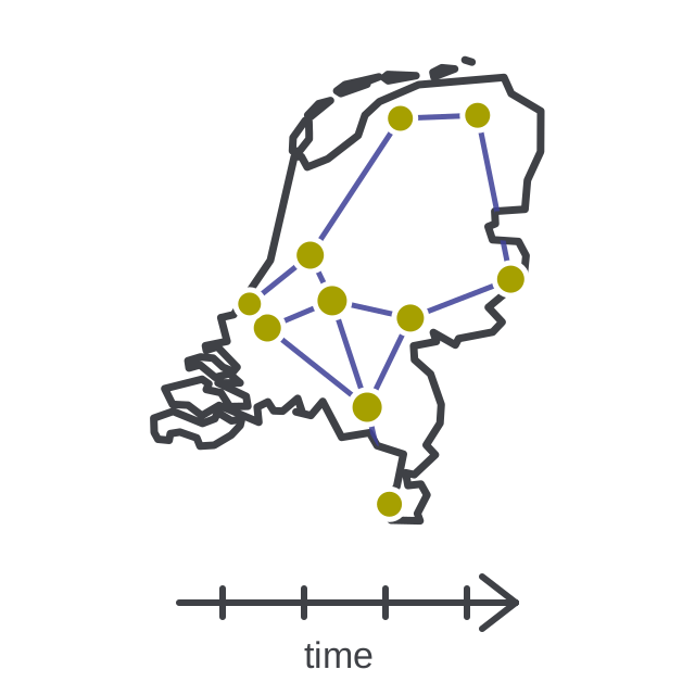
Geospatial Projects

• Project name: landuse_analysis
• Research question: What is the relation between municipal land use and population composition?
• Programming language: R (suggested) or python (allowed)
• Expert contact: TBD, Marco Helvich

Canonical course conventions live in project_guidelines.md. That file is the source of truth for the four required workflow files (week1_explore.qmd, week2_operationalize_clean.qmd, week3_model.qmd, week4_storytelling.qmd), the data/model_data.rds -> data/model_results.rds pipeline, the raw-data policy, quality-check requirements, decision logs, and contribution tracking. Read it before starting and treat anything below as project-specific guidance on top of those conventions.

Tutorial framing

Geospatial data are complex because observations are tied to coordinate systems, geometric boundaries, raster surfaces, and spatial dependence rather than arriving as independent rows in a single analysis-ready table.

Students should learn three main things about these data:

1. How spatial data are represented through vector geometries, raster grids, coordinate reference systems, spatial identifiers, and formats or services such as GeoJSON, Shapefiles, GeoTIFF, WFS, and WMS.
2. How to turn raw spatial sources into an analysis-ready table through spatial joins, raster-to-polygon aggregation, transformations, and documented choices about what land use and population composition mean.
3. How spatial dependence affects modeling, visualization, assumptions, and interpretation, including when residual autocorrelation or SAR/CAR-style models matter.

Peer-teaching checklist

Dimension	This project teaches
Data structure	Vector geometries, raster grids, tabular attributes linked by spatial identifiers, and spatial adjacency graphs.
Storage system	File-based spatial datasets and geospatial web services from PDOK/CBS.
File formats	GeoJSON, Shapefile, GeoTIFF, and tabular exports such as CSV.
Encoding	JSON for GeoJSON, binary spatial files for Shapefile components and GeoTIFF, and CRS metadata.
Model	Linear or GLM baseline, residual spatial autocorrelation check, and SAR/CAR-style extension if needed.
Key aspects to explain	CRS, vector vs. raster data, WFS/WMS, spatial joins, raster-to-polygon aggregation, spatial dependence (Moran’s I, SAR/CAR when needed), and the Modifiable Areal Unit Problem (MAUP).

Resources

Data sources

• PDOK (Public services on the map), specifically:
  • Statistics Netherlands’ areal boundaries data
  • Wageningen university’s land-use data
• Statistics Netherlands core figures

Feel free to use different sources if you want.

Knowledge sources

• R packages sf and terra
• The book Geocomputation with R (e.g. chapter on raster-vector interactions and data I/O)
• Find your own resources on spatial autoregressive models: CAR.

Week-by-week

Week 1:

Start from raw spatial files or web services, identify the data generating process, and explain vector/raster or point/polygon structure before doing any modeling.

• What is the standard key identifier for municipalities in the Netherlands?
• Can we connect directly to PDOK from R to retrieve all municipalities’ boundaries? Or can we download the information?
• Can we connect to PDOK from R to retrieve land-use information?

Prepare for the roundtable of week 2:

• What is a CRS/coordinate reference system and why is it needed?
• What is the difference between vector and raster data?
• What is a web map service (WMS) and a web feature service (WFS)?
• What are the advantages of GeoJSON vs shapefiles?

Week 2

Operationalize the research question by turning raw geometry-linked files into one analysis table, and document why the data were stored in that format.

• How can we create a tidy dataset of municipalities with their land-use and population characteristics to perform statistical modeling?
• What, exactly, does land-use mean?
• What dimensions of population composition do we find relevant?

Prepare for the roundtable of week 3:

• Explain the main spatial operations: spatial joins, aggregation from grid or point data, etc.

Week 3:

Fit models, explain preprocessing decisions, and show one sensitivity check to spatial choices.

• Assuming regression-type model, what is/are the outcome(s) and which predictors?
• Do we need to do some transformations, what type, GLM? Or just linear model?
• Fit a baseline (non-spatial) model first, then test residual spatial dependence (e.g. Moran’s I on residuals). Only escalate to SAR/CAR if the baseline residuals show meaningful spatial structure.
• Which parameters, specifically, answer our research question?
• Sensitivity check: show one Modifiable Areal Unit Problem (MAUP) sensitivity — re-run the analysis at a different aggregation level (e.g. neighbourhood vs municipality) or with a different boundary definition, and report whether the conclusion changes.

Prepare for the roundtable of week 4:

• Explain how spatial dependencies impact ordinary i.i.d. modeling and how to detect them (Moran’s I, residual maps).
• If SAR/CAR was needed: explain at a high level how each handles spatial dependence and when you would prefer one over the other. If the baseline residuals were spatially independent, explain why SAR/CAR was not necessary and what would have changed if dependence had been present.
• Explain the Modifiable Areal Unit Problem (MAUP) and how aggregation/boundary choices can change a spatial result.
• Explain how to read a spatial result: what the map, coefficient, or residual pattern is actually showing.
• Explain how sensitive conclusions can be to some of the decisions you took.

Week 4:

Visualize and tell a story

• What is the context? What is the main result? Why is it important?
• Which visualizations support our research findings?
• What are the assumptions and limitations of your design?